Numerische Lösungen der stationären SGL
Numerisches Probierprogramm (Euler-Cauchy)
| > | restart: |
| > | inte:=proc() global x,u,us: uss:=-c*(E-V(x))*u; us:=us+uss*dx; u:=u+us*dx; x:=x+dx; u; end; |
Warning, `uss` is implicitly declared local to procedure `inte`
![]()
| > | V:=x->a*x^2/2; |
![]()
| > | a,x,u,us,c,E,dx:=0.8/2/1.6022e-19,0,0,1,1.6022e-19*1.638e38,4.1434,5e-12; |
| > | for i to 500 do up[i]:=inte() od: |
| > | plot([seq([i,up[i]],i=1..500)],0..500); |
![]()
![[Maple Plot]](images/schroenum4.gif)
| > |
Es gibt eine Reihe von Möglichkeiten die numerischen Lösungen mit dsolve und odeplot darzustellen. (Das ist aber nicht sehr flexibel...)
| > | restart:with(plots): |
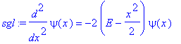
| > | sgl:=diff(psi(x),x$2)=-2*(E-x^2/2)*psi(x); |
| > | sol:='sol': |
| > | sol:=dsolve({subs(E=7/2,sgl),psi(0)=0,D(psi)(0)=1},numeric); |
| > | sol(1); |
![]()
| > | odeplot(sol,-5..5,numpoints=200); |
![[Maple Plot]](images/schroenum12.gif)
Funktion zur Übergabe von E (Randwerte müssen im folgenden Befehl eingegeben werden und sind dann fest):
| > | solE:=Evar->dsolve({subs(E=Evar,sgl),psi(0)=0,D(psi)(0)=1},numeric); |
![]()
| > | solE(7/2)(1); |
![]()
| > | odeplot(solE(11/2),-5..5,numpoints=200); |
![[Maple Plot]](images/schroenum15.gif)
| > |
| > | display([seq(odeplot(solE(E),-5..5,numpoints=200),E=1..2)],view=[-5..5,-1..1]); |
![[Maple Plot]](images/schroenum16.gif)
| > |
Animation mit E als Parameter
| > | display([seq(odeplot(solE(E),-5..5,numpoints=200),E=seq(1/2+i/5,i=0..50))],view=[-5..5,-1..1],insequence=true); |
![[Maple Plot]](images/schroenum17.gif)
| > |
Variabler x-Wert für Randwert. Hintergrund: Man sollte mit der numerischen Lösung an beliebiger Stelle beginnen können - für geeignete Darstellungen, aber auch wegen Konvergenzfragen. (Mit symbolischen Lösungen ist das ziemlich kompliziert - wenn man auch noch beliebige Potentiale verarbeiten will)
| > | solEx0:=(Evar,x0)->dsolve({subs(E=Evar,sgl),psi(x0)=0.001,D(psi)(x0)=0.001},numeric); |
![]()
| > |
| > | solEx0(7/2,-4)(1); |
![]()
| > |
Animation, in der der Randwert der Energie angepasst ist
| > | display([seq(odeplot(solEx0(E,-sqrt(2*E)*1.1),-5..5,numpoints=200),E=seq(1/2+i/5,i=0..100))],view=[-5..5,-0.01..0.01],insequence=true); |
![[Maple Plot]](images/schroenum20.gif)
| > |
Komplette Eingabe von Energie und Randwerten
| > | solEpar:=(Evar,x0,x0w,dx0,dx0w)->dsolve({subs(E=Evar,sgl),psi(x0)=x0w,D(psi)(dx0)=dx0w},numeric); |
![]()
| > | solEpar(7/2,0,0,0,1)(1); |
![]()
Plot
| > | plot([seq(psil(E,-sqrt(2*E)*1.1,0.01,-sqrt(2*E)*1.1,0.01)(x)^2*2000+E,E=seq(1/2+i/20,i=0..50)),x^2/2],x=-3..3,0..4); |
![[Maple Plot]](images/schroenum34.gif)
Animation
![[Maple Plot]](images/schroenum36.gif)
komma@oe.uni-tuebingen.de